Dynamic quantum qtates
The famous time-dependent Schrodinger equation has eluded physicists for years.
In these calculations we must consider uncertainty between position, momentum, energy, and time. Here is the general probability density solution to the above equation.

The first sum contains terms from the stationary state, time-independent solution. In quantum dynamics the second sum becomes non zero revealing coherence.
The left side of figure 1 below we have a quantum harmonic oscillator system as a linear combination of time-dependent states in position space. This is apperant in the energy having an uncertainty from about n=2 to n=5. On the left the uncertainty in position is depicted as a broad band. When the uncertainty in energy and position overlap they create a colored representation of the uncertainty in the position and the energy at the same time. As expected, the red lines are the expectation values for the energy and position. The position and energy expectation values and uncertainties are at a snapshot in time as they can oscillate around equilibrium, being a non-stationary state.
The right side of figure 1 below is again a quantum harmonic oscillator system as a linear combination of time-dependent states in momentum space. The energy uncertainty again ranges from about n=2 to n=5. On the left the uncertainty in position is depicted as a broad band. When the uncertainty in energy and momentum overlap they create a colored representation of the uncertainty in the momentum and the energy at the same time. As expected, the red lines are the expectation values for the energy and position. The energy and momentum expectation values and uncertainties are at a snapshot in time as they can oscillate around equilibrium, being a non-stationary state.
Figure 1
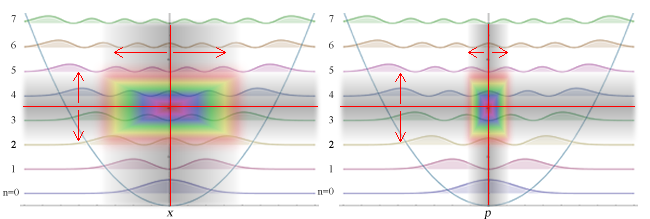
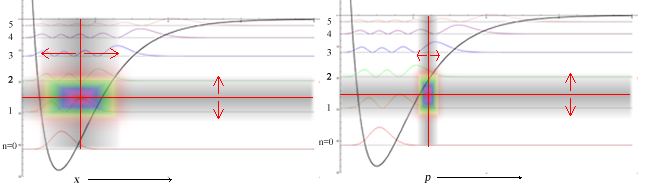
Figure 2 we have a quantum anharmonic oscillator system as a linear combination of time-dependent states. Again, the energy uncertainties for position and momentum should be the same, somewhere between n=1 and n=2. The expectation values oscillate back and forth in the colored overlap areas periodically obeying the Heisenberg uncertainty principle. A key distinguishing factor between stationary and non-stationary states is now expectation values and uncertainties of position, momentum, energy, and hence time, are able to oscillate around equilibrium.
Figure 2
Paul Falstad wrote an applet that clearly demonstrates coherence in quantum mechanics: Morse Modified Faulstad Applet
The animations from Wikipedia entries are very clear as well.
 |
 |
|
A harmonic oscillator in classical mechanics (A-B) and quantum mechanics (C-H). In (A-B), a ball, attached to a spring, oscillates back and forth. (C-H) are six solutions to the Schrödinger Equation for this situation. The horizontal axis is position, the vertical axis is the real part (blue) or imaginary part (red) of the wavefunction. (C,D,E,F), but not (G,H), are stationary states, or standing waves. The standing-wave oscillation frequency, times Planck's constant, is the energy of the state. |
Three wavefunction solutions to the Time-Dependent Schrödinger equation for a harmonic oscillator. Left: The real part (blue) and imaginary part (red) of the wavefunction. Right: The probability of finding the particle at a certain position. The top two rows are two stationary states, and the bottom is the superposition state, which is not a stationary state. The right column illustrates why stationary states are called "stationary". |